Lab 3 - Structure from Motion
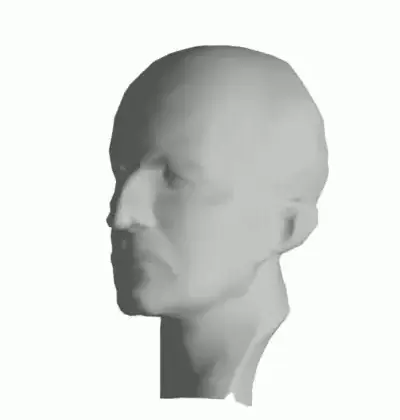
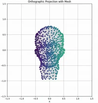
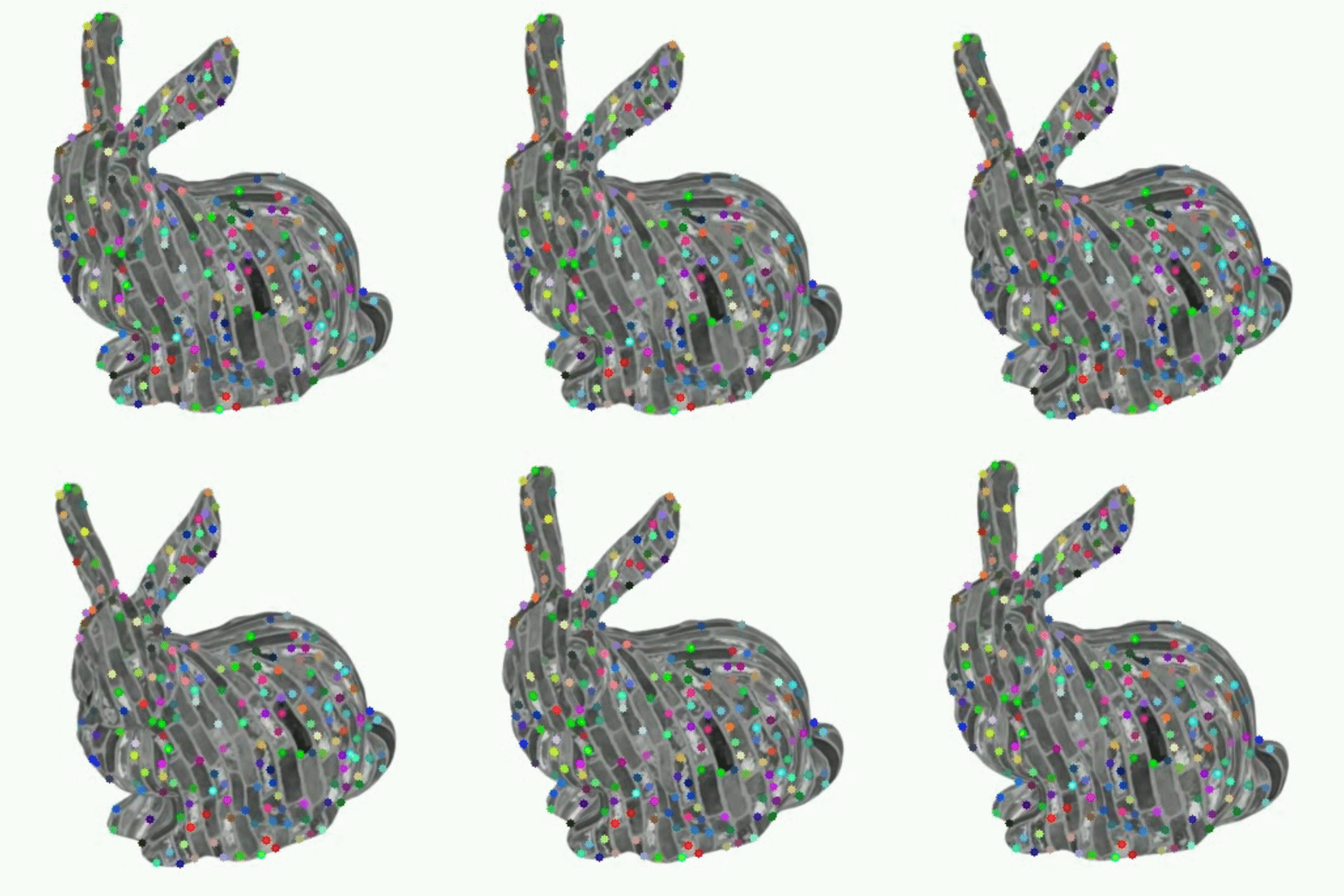
Middle: Sequence of tracked feature points on ground truth mesh viewed from an orthographic camera.
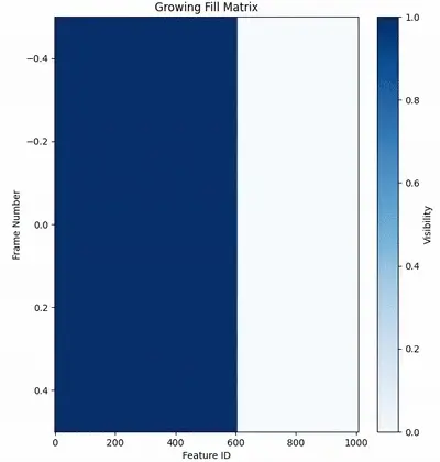
Right: Fill matrix visualization showing gradual accumulation of observations across frames (shaded entries are known image coordinates).
Overview
In this assignment you will implement an affine factorization method for structure from motion. You will then extend it to perform a metric upgrade to recover the true Euclidean structure. You will test your implementation on provided datasets and on your own videos, and document your results with code, figures, and analysis.
Important: You can obtain 2 bonus marks for each section you finish and demo while present during the lab period we introduce the lab.
Lab Introduction Slides: available here
Prelab Questions (5%)
The link to the prelab questions can be found here. You will need your University of Alberta email for access; they are also available under the Canvas assignment. Due Tuesday, March 3rd at 5pm.
Setup
First, download the lab code and report templates. These contain the structure for your report, and the file structure for your code. You can write your code however you wish within the files; however, please ensure that it is adequately commented, and that each part of the lab can be run by running the file corresponding to that question.
You will need to use your University of Alberta email to access the below templates.
Code template: can be found here.
Report template: can be found here.
1: Affine Factorization Method (45)
Background: The affine factorization algorithm (described in Section 18.2 in Hartley & Zisserman, 2nd ed.) implements the Tomasi–Kanade method for Structure from Motion under an orthographic projection assumption.
The key insight is that when tracking \(P\) feature points across \(F\) frames (views), the resulting \(2F \times P\) measurement matrix will have rank 3 for a rigid scene under orthographic projection, after proper normalization (centering). This matrix can be factored into motion and shape matrices via Singular Value Decomposition (SVD).
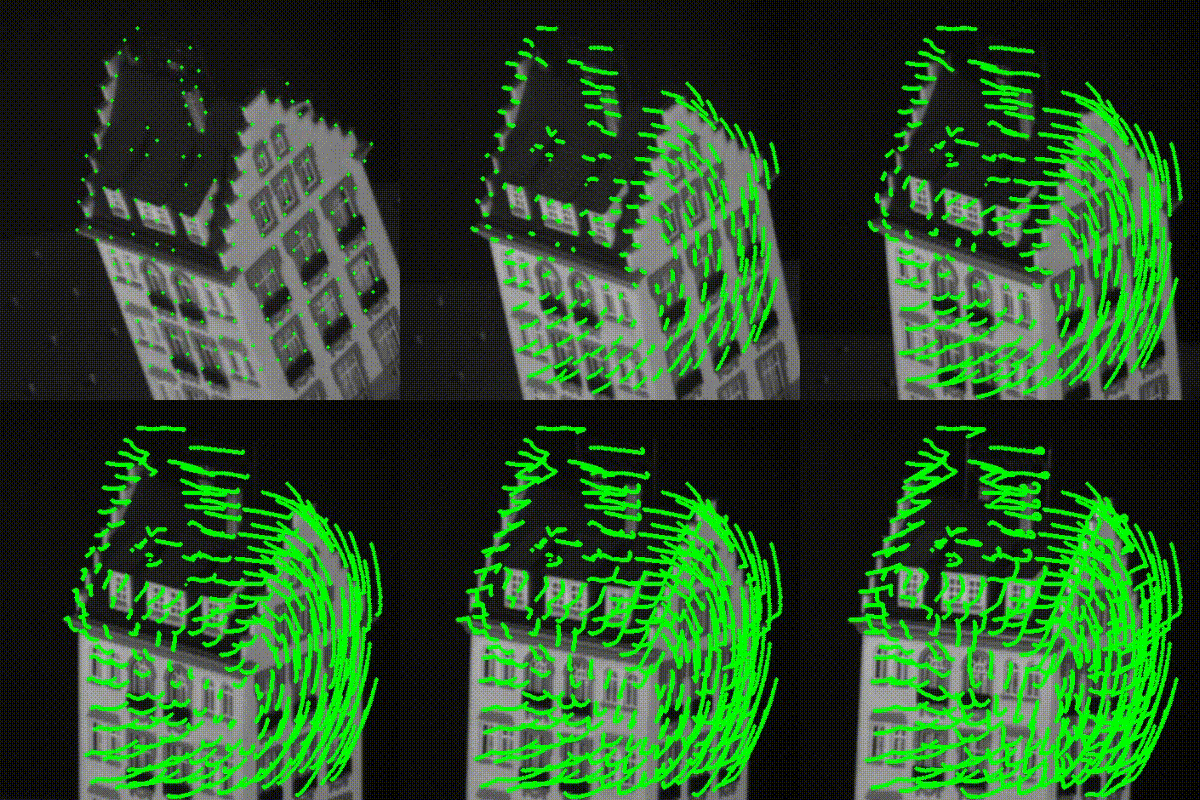
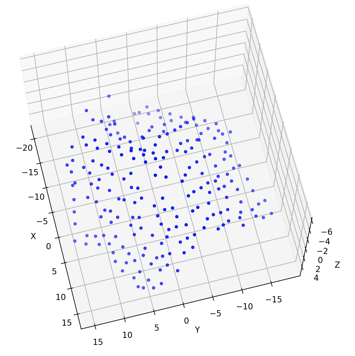
Right: Example of a 3D reconstruction output.
Task:
Implement the affine structure-from-motion algorithm following the procedure from Lecture 07 (slides 27–30) or the textbook on the following two datasets:
- The hotel dataset found here. In the zip, the measurement matrix can be found in the .txt.
- A short video you record yourself. You may use feature_tracker.py which finds good feature points, tracks them, and performs a global optimization to refine the tracking if you wish.
-
Form the measurement matrix \(W\) using tracked feature coordinates:
- Normalize the data by subtracting the mean from each row (i.e., each image’s \(x\) and \(y\) coordinates)
- This centering removes the translational motion and ensures \(W\) is of rank 3 in the noise-free case
-
Perform singular value decomposition: \(W \approx U \Sigma V^T\)
- Take the top 3 singular values and corresponding vectors (because the ideal rank is 3)
- Extract \(U_0\) (size \(2F \times 3\)), \(\Sigma_0\) (\(3 \times 3\)), and \(V_0\) (\(P \times 3\))
-
Factor into motion and shape matrices:
- Initialize the motion matrix as \(R = U_0 \Sigma_0^{1/2}\)
- Initialize the shape matrix as \(S = \Sigma_0^{1/2} V_0^T\)
At this point, \(W \approx R S\) gives an affine reconstruction of the cameras (in \(R\)) and 3D points (in \(S\)). Note that this reconstruction is not unique – any \(3 \times 3\) invertible transform \(Q\) gives an equivalent solution \(RQ\) and \(Q^{-1}S\).
Deliverables:
For each dataset (hotel and your own), save the following figures to include in your code submission and display them in your report:
- Plot the recovered 3D point cloud (obtained from \(S\))
Extra Tools and Resources:
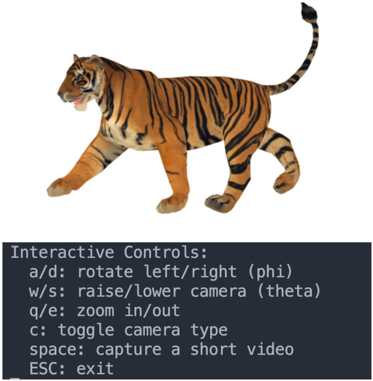
- capture_motion.py is a python script that generates video data from a textured 3D mesh. Terminal inputs allow for control recording and the view of the model.
- Textured 3D models can be found here
Report Question 1:
In your report, discuss what happens when applying this method to your own video data. Note that real cameras are projective, not orthographic, so your method might not perfectly reconstruct real video data. Analyze the differences and limitations you observe.
2: Metric Upgrade; Euclidean Reconstruction (40)
The factorization method you implemented in Part 1 yields a reconstruction that is affine – meaning it’s determined only up to an arbitrary linear transformation in 3D space. To recover the true Euclidean structure (up to a scale factor), we need to enforce that camera motions correspond to orthonormal rotations. This refinement process is known as the metric upgrade or affine to metric calibration.
In this question, you will implement the metric upgrade procedure to transform your affine reconstruction into a Euclidean one. You will then use a known scale factor between feature points to properly scale your reconstructed model to real-world dimensions.
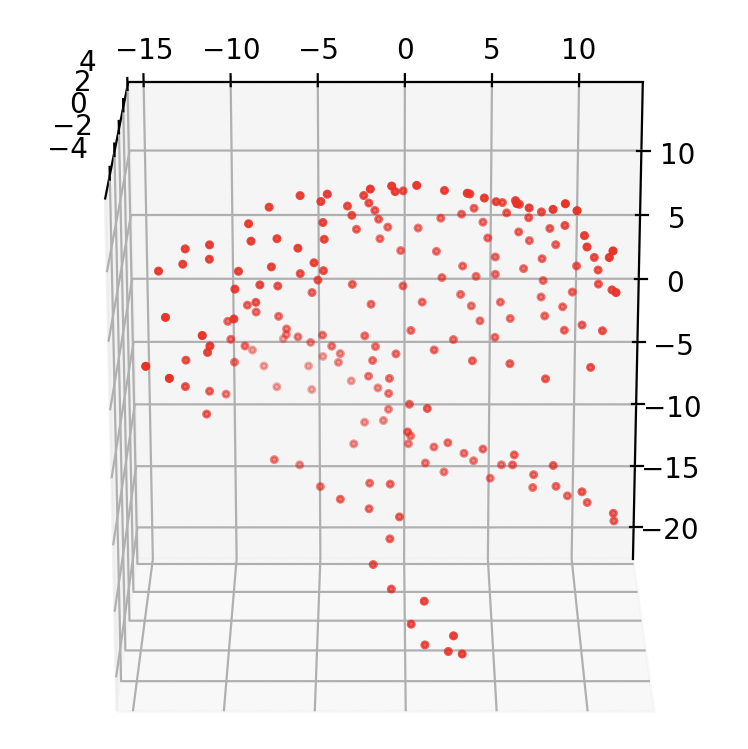
Right: Resulting Euclidean reconstruction.
a) Derive the Orthonormality Constraints
Suppose the \(i\)-th camera has affine motion represented by the two 3D row vectors \(r_{i1}\) and \(r_{i2}\) (from the \(R\) matrix). For a real rotation, we require: \(\begin{align} r_{i1} \cdot r_{i1}^T &= 1 \\ r_{i2} \cdot r_{i2}^T &= 1 \\ r_{i1} \cdot r_{i2}^T &= 0 \end{align}\) These constraints can be written in terms of the unknown metric upgrade matrix \(L = QQ^T\) (a symmetric \(3\times3\) matrix):
- For the first constraint: \(r_{i1} L r_{i1}^T = 1\)
- For the second constraint: \(r_{i2} L r_{i2}^T = 1\)
- For the third constraint: \(r_{i1} L r_{i2}^T = 0\)
Write out these equations for all cameras, resulting in at most \(3F\) equations (3 per frame) for the 6 independent entries of \(L\) (since \(L\) is symmetric).
b) Solve for the Upgrade Matrix
Arrange the constraints into a linear system \(AL = b\) where:
- \(A\) is a matrix containing coefficients from the constraints
- \(L\) is a vector of the 6 independent entries of the symmetric matrix \(L\)
- \(b\) is a vector with entries 1, 1, 0, … for each camera’s constraints
Solve this system using linear least-squares to find the \(L\) that best satisfies all equations.
c). Compute the Upgrade Transformation
Once you have \(L \approx QQ^T\):
- Perform a Cholesky decomposition or eigen-decomposition to obtain \(Q\)
- You may need to create a positive definite approximation if \(L\) has negative or zero eigenvalues due to noise
- One approach is to perform eigen-decomposition, set any negative eigenvalues to a small positive value, and reconstruct \(L\)
- Apply \(Q\) to the affine reconstruction to get the Euclidean reconstruction:
Now \(R_{\text{euclid}}\) should represent valid rotation matrices (scaled) and \(S_{\text{euclid}}\) is the structure in Euclidean space (up to an overall scale factor).
d) Apply Absolute Scale Calibration
To obtain a model with real-world dimensions, you need to use known physical measurements between feature points. Use The figure below to calibrate the scale of your Hotel reconstruction from Part 1:
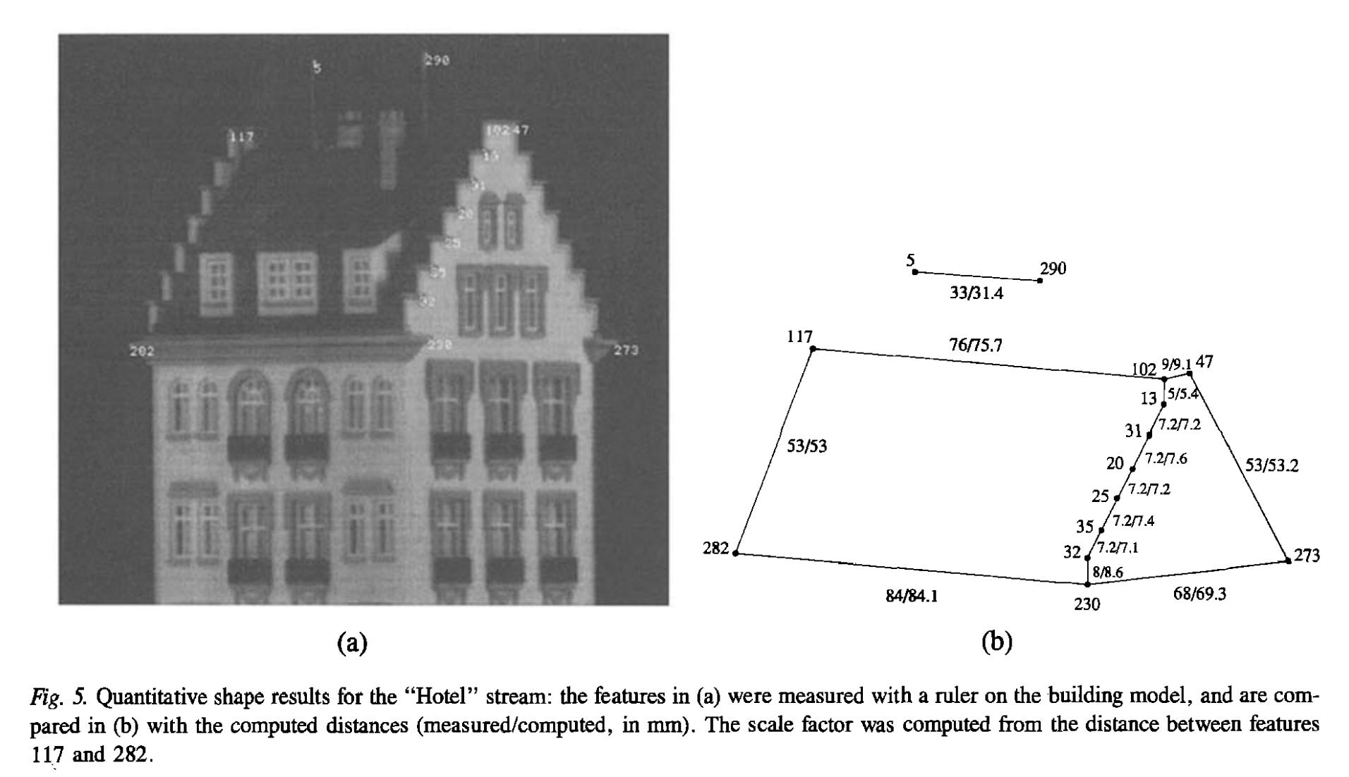
- Identify reference points: Select two or more feature points in your reconstruction where you know the actual physical distance between them. For example:
-
Compute the scale factor:
- Let \(d_{real}\) be the known real-world distance between your reference points
- Let \(d_{recon}\) be the corresponding distance in your reconstructed model
- The scale factor is then \(s = d_{real} / d_{recon}\)
-
Apply the scale:
- Scale your Euclidean reconstruction: \(S_{scaled} = s \times S_{euclid}\)
-
Verification:
- Measure other known distances in your scaled model to verify the accuracy
Your final scaled reconstruction should now have proper real-world dimensions, allowing for ‘accurate’ measurements and integration with other 3D models or systems.
Deliverables:
Using the provided Hotel data, save the following figures to include in your code submission and display them in your report:
- Plot the recovered 3D point cloud (obtained from \(S\))
- Evaluate its accuracy
Report Question 2:
Visualize the 3D reconstruction before and after the metric upgrade. Analyze, using your own methods, how the metric upgrade affects the quality of the reconstruction. How good are your between reconstructed distances compaird to the known distances?
e) Metric upgrade on your own data
Now we will perform the same metric upgrade on your own video data.
Deliverables:
Record two different video sequences to run through your affine reconstruction pipeline. These can use the same or different objects; one of them can be the video you captured for Question 1.
One of your videos should lead to a successful reconstruction, and the other should result in a poor reconstruction.
For each video:
- Plot the recovered 3D point cloud from your video (obtained from \(S\))
- Evaluate its accuracy
For your poor reconstruction video, do not simply shake the camera, or make other violent motions/lighting changes that lead to complete tracking failure. The goal is not to evaluate tracking, but your reconstruction algorithm, and to understand what kinds of camera motion or capturing scenarios can lead to failure.
Report Question 3a): In your successful reconstruction, what kind of camera motion did you use? Why is this movement appropriate?
Report Question 3b): In your poor reconstruction, what kind of camera motion did you use? Why does this cause the reconstruction to fail?
3: Meshing and Texturing (15)
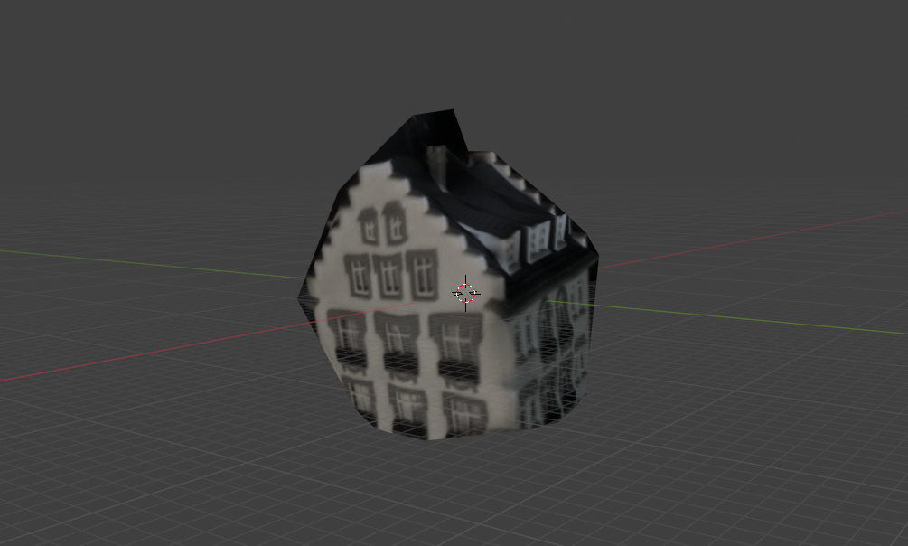
Now that we have a euclidean reconstruction, we can turn it into a 3D mesh and texture it to create a rough 3D model of our object. We will use a simple approach to this. Given a single image from our dataset, we first can triangulate our points to create a mesh, which we can then texture by mapping pixels in an image to the vertices of our mesh triangles. We will then create a .obj file containing our mesh.
To simplify this process, we will make use of libraries for triangulation and 3D geometry. Specifically we will need scipy and open3d, which can be installed by pip install scipy open3d.
The file q3_texturing.py contains a partially completed function save_textured_mesh() which creates a mesh given your 3D reconstructed points, and an image with its corresponding 2D points. It also contains code for saving the mesh as an obj.
However, this function is missing the texture mapping, which tells the mesh where in the image to look for the texture of each triangle. Your job is to complete this part of the code, and then use it to generate a mesh for both the hotel data and your own data. You need to:
- Create a vector to store the (u,v) texture coordinates for each point of each triangle
- Fill in the (u,v) coordinats for each point, normalized to 0-1 range, where (0, 0) is the bottom left corner.
This function will save your mesh as a .obj file, with an accompanying .png for the texture image, and a .mtl file that specifies the material properties for the obj. These can be viewed in a standard 3D viewer such as blender, or a online at https://3dviewer.net/.
Deliverables:
- Include the
.obj,.mtl, and.pngfiles for each mesh in your media folder. - Include an image of your meshes in your report.
Report Question 4a): How does the quality of your reconstruction affect the final mesh?
Report Question 4b): Which frame did you choose for your texture image? How might this choice affect your result?
Bonus (10) - Triangulation
- Implement your own triangulation procedure, rather than using the provided
scipy.spatial.Delaunay. You likely will need to modify other parts of thesave_textured_meshfunction if you choose to do this. Using an alternate library for triangulation would not count for this question.
Deliverables:
- Describe how your triangulation procedure works in your report.
Bonus (10) - Alternate Meshing
- Use another algorithm to mesh one of your resulting 3D point clouds and include it in your code submission (media folder) and report. Describe the meshing algorithm you implemented or library you utilized (e.g., Ball-Pivoting, Poisson Surface Reconstruction, Alpha Shapes). Explain why you selected this particular meshing approach and its suitability for the structure-from-motion point clouds.
Deliverables:
- Include the resulting mesh in your report, as well as your discussion of your meshing approach.
Submission Details
- Include accompanying code used to complete each question. Ensure they are adequately commented.
- Ensure all functions are and sections are clearly labeled in your report to match the tasks and deliverables outlined in the lab.
- Organize files as follows:
-
code/folder containing all scripts used in the assignment. -
media/folder for images, videos, and results.
-
- Final submission format: a single zip file named
CompVisW26_lab3_lastname_firstname.zipcontaining the above structure. - Your report for Lab 3 is to be submitted at a later date. The report contains all media, results, and answers as specified in the instructions above. Ensure your answers are concise and directly address the questions.
- Total marks for this lab is 100 for all students. Your lab assignment grade with bonus marks is capped at 110%.