Lab 2.1 - 2D Projective Geometry and Homography Estimation
Overview
In this lab you’ll learn about 2D projective geometry and homography estimation.
Lab Introduction Slides: available here
Important: You can obtain 1 bonus mark for each section you finish and demo while present during the lab period we introduce the lab.
Prelab Questions (5%)
The link to the prelab questions can be found here. You will need your University of Alberta email for access; they are also available under the Canvas assignment. Due Tuesday, Feburary 3rd at 5pm.
Setup
First, download the lab code and report templates. These contain the structure for your report, and the file structure for your code. You can write your code however you wish within the files; however, please ensure that it is adequately commented, and that each part of the lab can be run by running the file corresponding to that question.
You will need to use your University of Alberta email to access the below templates.
Code template: can be found here.
Report template: can be found here.
1. Homogeneous Transforms (20)
A transformatrion matrix, \(M\), can be used to transform 2D points in homogeneous form:
\begin{equation} \left(\begin{array}{l} \displaylines{x’\\ y’\\ w} \end{array}\right) = M \left(\begin{array}{l} \displaylines{x\\ y\\ 1} \end{array}\right) \end{equation}
We define translation, rotation, scale and shear matricies in homogenenous coordinates as follows:
\begin{equation} T=\left[\begin{array}{ccc} \displaylines{ 1 & 0 & t_x\\ 0 & 1 & t_y\\ 0 & 0 & 1 } \end{array}\right] \end{equation}
\begin{equation} R=\left[\begin{array}{ccc} \displaylines{ cos\theta & -sin\theta & 0\\ sin\theta & cos\theta & 0\\ 0 & 0 & 1 } \end{array}\right] \end{equation}
\begin{equation} S=\left[\begin{array}{ccc} \displaylines{ s_x & 0 & 0\\ 0 & s_y & 0\\ 0 & 0 & 1 } \end{array}\right] \end{equation}
\begin{equation} Sh=\left[\begin{array}{ccc} \displaylines{ 1 & sh_x & 0\\ sh_y & 1 & 0\\ 0 & 0 & 1 } \end{array}\right] \end{equation}
These matrices transform the homogeneous points with respect to the coordinate origin. They can be multiplied in any order and order of multiplication determines the order of the transformations performed on the points. For further reading, see Chapter 2.4 of Hartley and Zisserman.
The following code loads the point cloud house.npy and displays it in a 2d scatterplot. Use these points to complete Question 1. You must add the homogeneous coordinate row yourself.
house.txt is also available if you prefer. Use np.loadtxt() with delimiter=',' to load it.
with open('happy.npy', 'rb') as f:
    house = np.load(f, allow_pickle=True)

fig = plt.figure()
ax = fig.add_subplot()
plt.scatter(house[0], house[1], color='gray')
ax.set_aspect('equal', 'box')
plt.title("House")
plt.show()
a) 2D Homogeneous Transformations
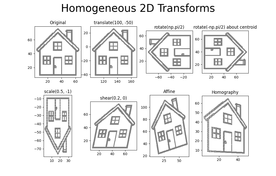
- Create functions that create translation, rotation, scale and shear transformation matricies using the equations provided above. Apply the following transformations to our provided house point cloud and recreate the above figure (with subplots).
- Original Point Cloud.
- Translate by (100, -50).
- Rotate by +90 degrees.
- Rotate by -90 degrees about centroid.
- Scale by (0.5, -1).
- Shear by (0.2, 0).
- Affine transformation given
Affine = np.array([[0.9, -0.2, 10], [0.3, 1.2, 10]]). - Homography transformation given
Homography = np.array([[1, 0, 0], [0, 1, 0], [0.005, 0, 1]]). Ensure you divide all points by the homogeneous coordinate after applying the transformation.
- You will lose marks if your house is not at the same coordinates as our figure.
Deliverables:
- Save your figure to include with your submission.
- Display the image in your report.
Report Question 1a: What group of transformations do translation, rotation, scale and shear belong to? Name two ways these transformations differ from projective (homography) transforms?
b) Create a composite image

- Using a homography transform and our provided point cloud, approximately recreate the above image.
Deliverables:
- Display the image in your report.
- Save your image to include with your submission.
Report Question 1b: Describe how you created this image and the transformations you used.
c) Bonus (5) - Adding your own assets
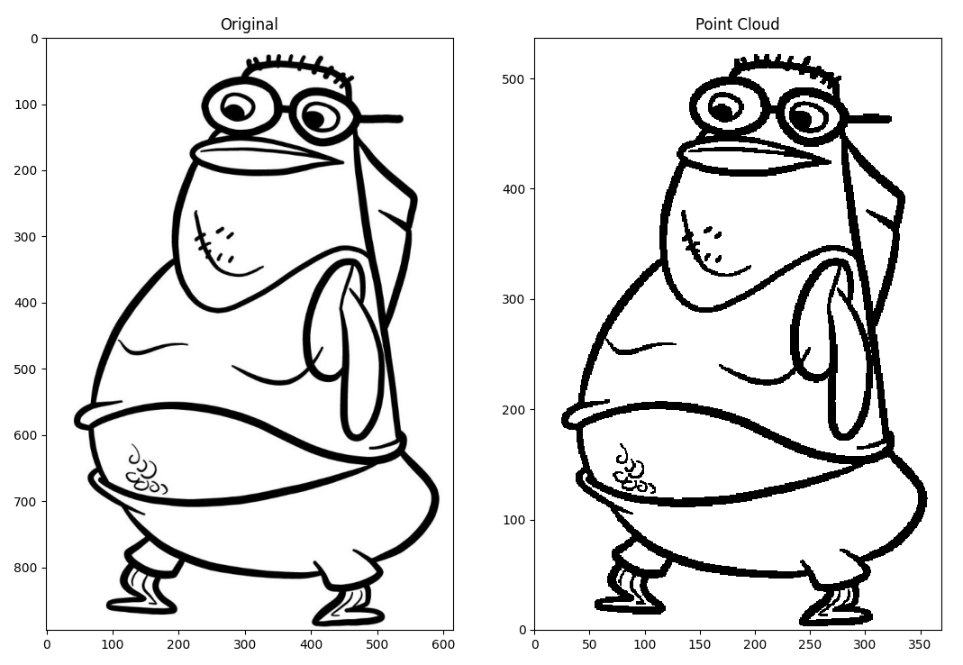
- Use the code on this page to generate point clouds of your own assets. Search up coloring page versions of your favorite characters and load them in.
- Create a composite image of your own using the transformations you’ve learned. Load in at least two assets and transform them to create a scene.
- Note: Large images can create tens of thousands of points. If it hampers performance reduce the number of points using
scale. - Make sure to find and use your own assets for this question!
Deliverables:
- Display the image in your report.
- Save your image to include with your submission.
Report Question 1c: Describe how you created this image and the transformations you used.
2. 2D Projective Geometry: Points, lines and their incidence (20)
a) Hand Drawing
The homogeneous equation of a line is given as follows: \begin{equation} l^Tx=ax+by+c=0 \end{equation} It holds true for all points that lie on the line.
The following three homogeneous lines display a simplified diagram of a railway track and the horizon.
\[l_1=\left(\begin{array}{c} 10 \\ -1 \\ 10 \end{array}\right) \quad l_2=\left(\begin{array}{c} -10 \\ -1 \\ 10 \end{array}\right) \quad l_H=\left(\begin{array}{c} 0 \\ 1 \\ -10 \end{array}\right)\]Sketch the drawing labelling all three lines and the position of the vanishing point, the intersection of \(l_1\) and \(l_2\), given by \(l_1\times l_2\).
Deliverables:
- Display the sketch in your report (you may use software like paint to draw this sketch or scan a hand sketch; 0 marks will be awarded for plots).
- Save the sketch to include with your submission.
b) Construct the midpoint and midline of the football field in the image below.
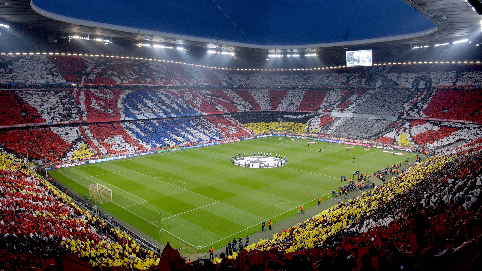
- Click on the corners of the field using
matplotlib.pyplot.ginput()or your own mouse callback. - Convert the points to homogeneous coordinates.
- Compute the diagonal lines \(l_1\) and \(l_2\) (the line between two points is \(l=p_1\times p_2\)).
- Compute the midpoint, \(p_m\) using the diagonal lines (the intersection between two lines is \(p=l_1\times l_2\)).
- Compute the vanishing point, \(p_\infty\) as the intersection of the two short sides of the field.
- Compute the midline using the vanishing point and the mid-point.
Deliverables:
- Display the image with overlaid features in your report.
- Save the image with overlaid features to include with your submission.
c) Bonus (10) - Construct the midpoint and midline on a video sequence
- Place a book with a textured cover on a table and record a video.
- Track the four corners of the book using 4 trackers, initialized by mouse clicks. You can use your own tracker or one of openCV’s built in trackers (CSRT is suitable, see resource on other openCV trackers).
- Use the tracked positions to draw the midline and midpoint on the book.
Deliverables:
- Save the video with overlaid features to include with your submission.
3. Robot Visual Servoing Task Specifications (20)
a) Line-to-line constraint
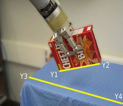
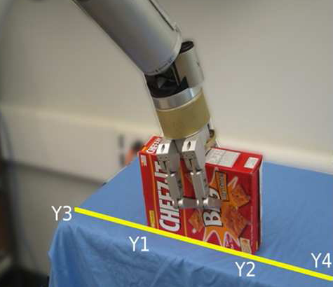
\begin{equation} e_{l2l} = y_1 \cdot (y_3 \times y_4) + y_2 \cdot (y_3 \times y_4) \end{equation}
- Create a live implementation of the line-to-line constraint.
- Place two box objects in the scene. Initialize the appropriate tracked points with mouse clicks to construct the line to line constraint.
- You may use openCV’s built in trackers (CSRT is suitable, see resource on other openCV trackers).
- Overlay the value of the constraint and the points/lines we are tracking onto the video (see
cv2.putText()). - Save a video with overlaid features. Rotate and move one of the books and bring the lines together.
- Optional: normalize the points and lines before computing the constraints to avoid overly large numbers.
Deliverables:
- Save the video with overlaid features to include with your submission.
- Display one frame of your video in your report.
Report Question 3a: What happens to the value of our constraint when we bring one line to the other?
b) Parallel lines constraint
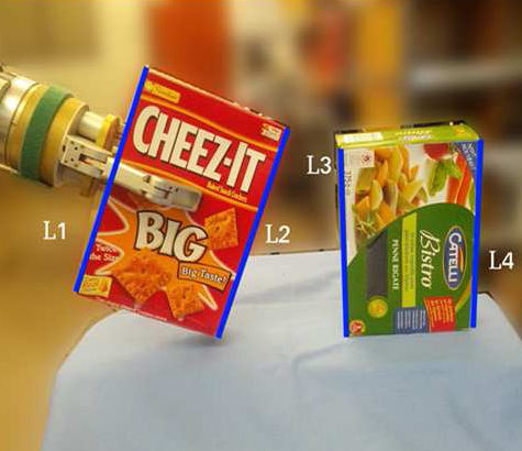
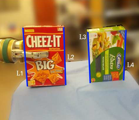
The equation for the line to line constraint is:
\begin{equation} e_{par} = (l_1 \times l_2) \times (l_3 \times l_4) \end{equation}
- Apply the same process in 3a) to make the parallel lines constraint. A live implementation is mandatory.
- The recorded video for this question should include rotations that change the sign of the parallel lines constraint.
- This time our constraint is vector valued. Overlay the constraint and the points/lines we are tracking onto the video and verify that its magnitude decreases when the books are near parallel, and its sign changes when the books cross the point of being parallel.
Deliverables:
- Save the video with overlaid features to include with your submission.
- Display one frame of your video in your report.
Report Question 3b: How can we use these constraints to control a robot?
4. Homography Estimation (40)
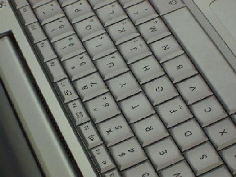
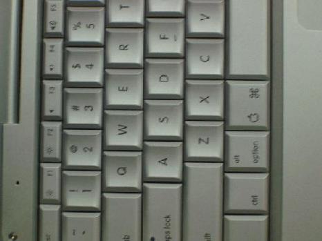
- See page 39-49 of these slides
- See sample results
a) Basic DLT Function
- Write a function
get_homography(x_1, x_2, normalization=False)that returns the homography matrix,H, between two images, given the 4 (or more) point correspondences,x_1andx_2between two images. - Apply your transformation to the first image to verify your results.
- Get the point correspondences through clicking on the same four features in two different images.
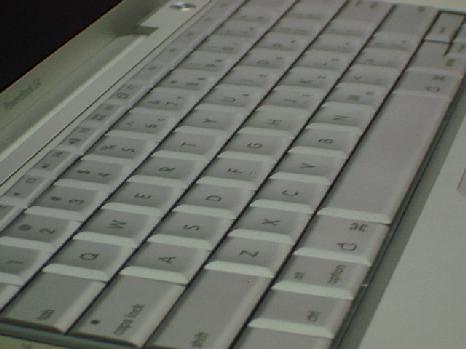
- You can use the keyboard images for testing - however, for submission, make sure you use your own images!
Deliverables:
- Display the two original images and the transformed image in your report.
Report Question 4a: What could be one real life use of this process?
b) Normalization
- Implement a normalization procedure into your algorithm. Translate the points such that their mean is centred at the origin. Scale the points such that the average norm of the distance to the origin is \(\sqrt 2\).
- Explore performance of your algorithm with your own pictures.
Deliverables:
- Using your own images, display the two originals and the transformed image in your report.
Report Question 4b: After the homography is applied, do the overlapping areas in the two images look exactly the same? Why or why not?
Report Question 4c: Correspondences are not always perfect. What happens if some of the correspondences are incorrect? How can this be handled?
5. Bonus (15) - Augmented Reality
- Track planar regions: Identify and track one or more four-point planar regions (e.g., a poster or book cover) in a video.
- Compute homography: Calculate the homography for each region.
- Project image: Warp an image (or images) onto the tracked surface so that, even as the camera moves, the projection remains fixed to the surface.
- Be creative! You can project onto trackable surface. An additional 5 bonus marks will be awarded cool-factor, as judged by the TAs.
Deliverables:
- Save the video with overlaid projections to include with your submission.
Submission Details
- Include accompanying code used to complete each question. Ensure they are adequately commented.
- Ensure all functions are and sections are clearly labeled in your report to match the tasks and deliverables outlined in the lab.
- Organize files as follows:
-
code/folder containing all scripts used in the assignment. -
media/folder for images, videos, and results.
-
- Final submission format: a single zip file named
CompVisW26_lab2.1_lastname_firstname.zipcontaining the above structure. - Your combined report for Lab 2.1 and 2.2 is to be submitted at the end of the topic at a later date. The report contains all media, results, and answers as specified in the instructions above. Ensure your answers are concise and directly address the questions.
- Total marks for this lab is 100 for all students. Your lab assignment grade with bonus marks is capped at 110%.