Note: We need to consider various normalization procedures. Refer to Algorithm 18.2 for details (page 445 of Hartley and Zisserman). I will also mention these in the lab.
(a). Implement the affine factorization algorithm described in section 18.2 or slides 27 to 30 of lec07 (5).
Test your implementation on the following data (each picture is a link to a data file):
 ,
,  ,
,
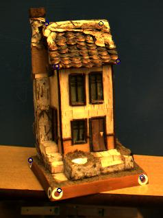
The first file, HouseTallBasler64.mat, contains an image sequence in the variable "mexVims". It also has image coordinates of tracked points in the matrix W arranged so that row indices indicate view number and column indices are point number. The first "NrFrames" rows are the x-coordinates, the next are y-coordinates. You can use the m-file plotHouse.m to see the files. If you are working at home you also need bayer2rgb.m. (This data was grabbed with the .m-file mexVTrackPtsGrabim2.m - this uses our obsolete software Mexvision that might not work on lab machines any more.)
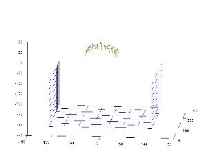
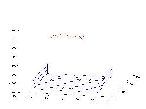
The other two sequences were synthetically generated. The images above show the 3D points, arranged on three planes and cameras. In the .mat files, W is organized identically as for the house and X contains the ground truth X coordinates.
Test your implementation on all three data sets (note that you have ground truth X, the 3-D coordinates, on the last two synthetic data sets).
(b) Use cameras and point trackers (e.g. from MTF) to reconstruct an object of your choice. (5)
(c) [bonus] Repeat (a) but this time implement the projective factorization method (i.e., estimate the scales iteratively). Refer to section 18.4 in Hartley and Zisserman or slides 32 to 35 in lec07. (bonus - 3)
- Compare the results you get in (a) and (c).
- Which one is "better", and in what sense?